Predicting US Census Data with XGBoost

Using US Census data to predict whether or not someone has an annual income of more than $50,000.

1 Introduction

This project is my final assignment for MAT-427: Statistical Machine Learning, where we were tasked with using data from the U.S. Census Bureau to predict whether or not someone earns more than $50,000 annually. This project is a hackathon, meaning I had to make trade-offs between accuracy and interpretability. Since accuracy is arguably most important in a hackathon, it was prioritized over interpretability (most evident in the “Final Thoughts” section).

1.1 Rationale

Since accuracy was my highest priority, I used gradient boosted trees (XGBoost in particular) for my model. XGBoost is widely used in competitive machine learning for its ability to efficiently model complex nonlinear relationships while handling missing data and feature interactions with minimal preprocessing.

2 Getting Started

tidymodels is the key package used.

library(tidyverse)
library(knitr)
library(tidymodels)
library(rpart.plot)
library(kableExtra)
library(stringr)
library(doParallel)
library(MASS)
library(wacolors)

tidymodels_prefer()

set.seed(427)

census_train <- read.csv("census_train.csv")
census_test <- read.csv("census_test.csv")

3 Data Visualization

3.1 Preparing Data for Visualization

We will use recipes and workflows to preprocess the data before modeling. Consequently, to not conflict with that, I made a copy of the training data for visualization purposes.

census_eda <- census_train

I made mild changes to our graphing data: I removed trailing whitespace, replaced ? values with Unknown, turned categorical variables into factors, and removed the inconsistent period at the end of some of the income values.

census_eda <- census_eda |>
  mutate(across(where(is.character), ~ str_trim(.))) |>
  mutate(across(where(is.character), ~ ifelse(. == "?", "Unknown", .))) |>
  mutate(across(where(is.character), as.factor)) |>
  mutate(income = as.factor(str_trim(str_replace_all(as.character(income), "\\.", ""))))

3.2 Finding the “Best” Predictors

I used feature selection to narrow our list of predictors to the most “meaningful” ones. To achieve this, I used stepwise selection (both forward and backward) and the BIC (Bayesian Information Criterion) to take a model with all predictors and return one with only the most impactful predictors.

eda_model <- glm(income ~ ., data = census_eda, family = binomial)
n <- nrow(census_eda) # get number of observations for BIC calculation
model_BIC <- stepAIC(eda_model, direction = "both", k = log(n), trace = FALSE)

Below, we can see the most impactful predictors:

formula(model_BIC)

income ~ age + workclass + fnlwgt + education + marital.status + 
    occupation + relationship + sex + capital.gain + capital.loss + 
    hours.per.week

3.3 Univariate Graph

Looking at the distribution of our response variable, we can see that most observations have an annual income of less than $50,000.

income_univariate <- ggplot(census_eda, aes(x = income)) +
        geom_bar(fill = "#412d5e", alpha = 0.9) +
        labs(
          title = "Distribution of Income",
          x = "Income",
          y = "Number of Observations") +
        theme_minimal() +
        theme(
          plot.caption = element_text(hjust = 0, size = 10),
          axis.text.x = element_text(angle = 45, hjust = 1)
          )

income_univariate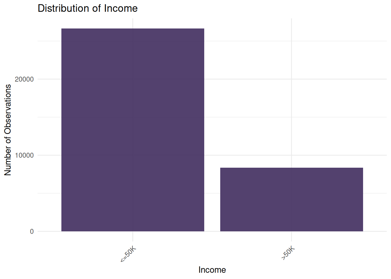

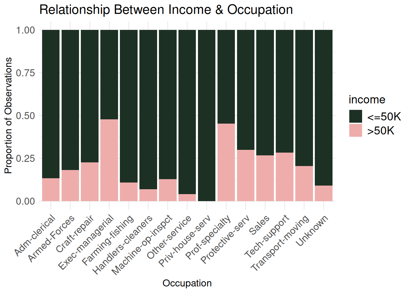
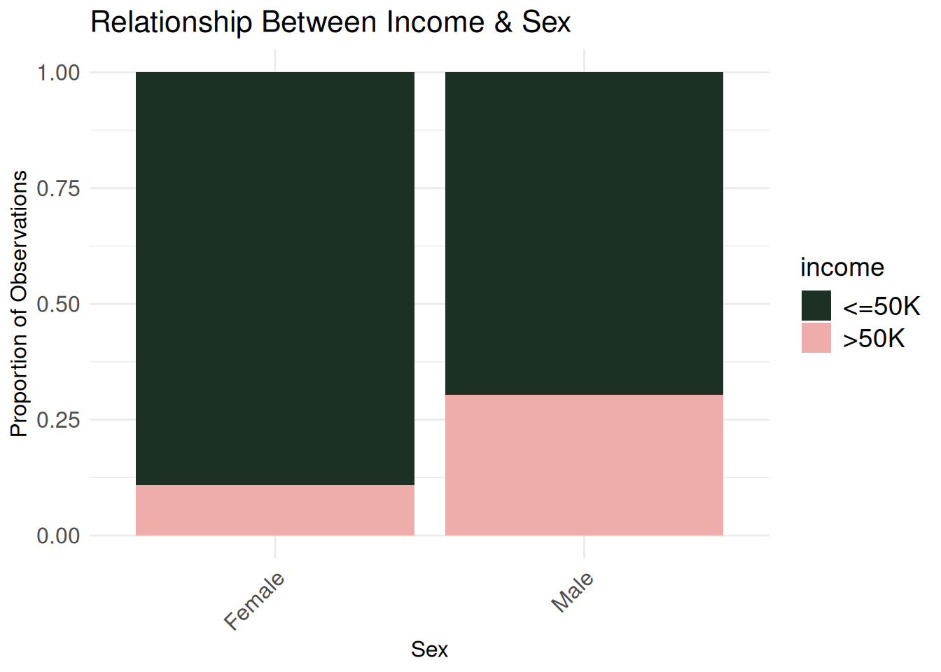
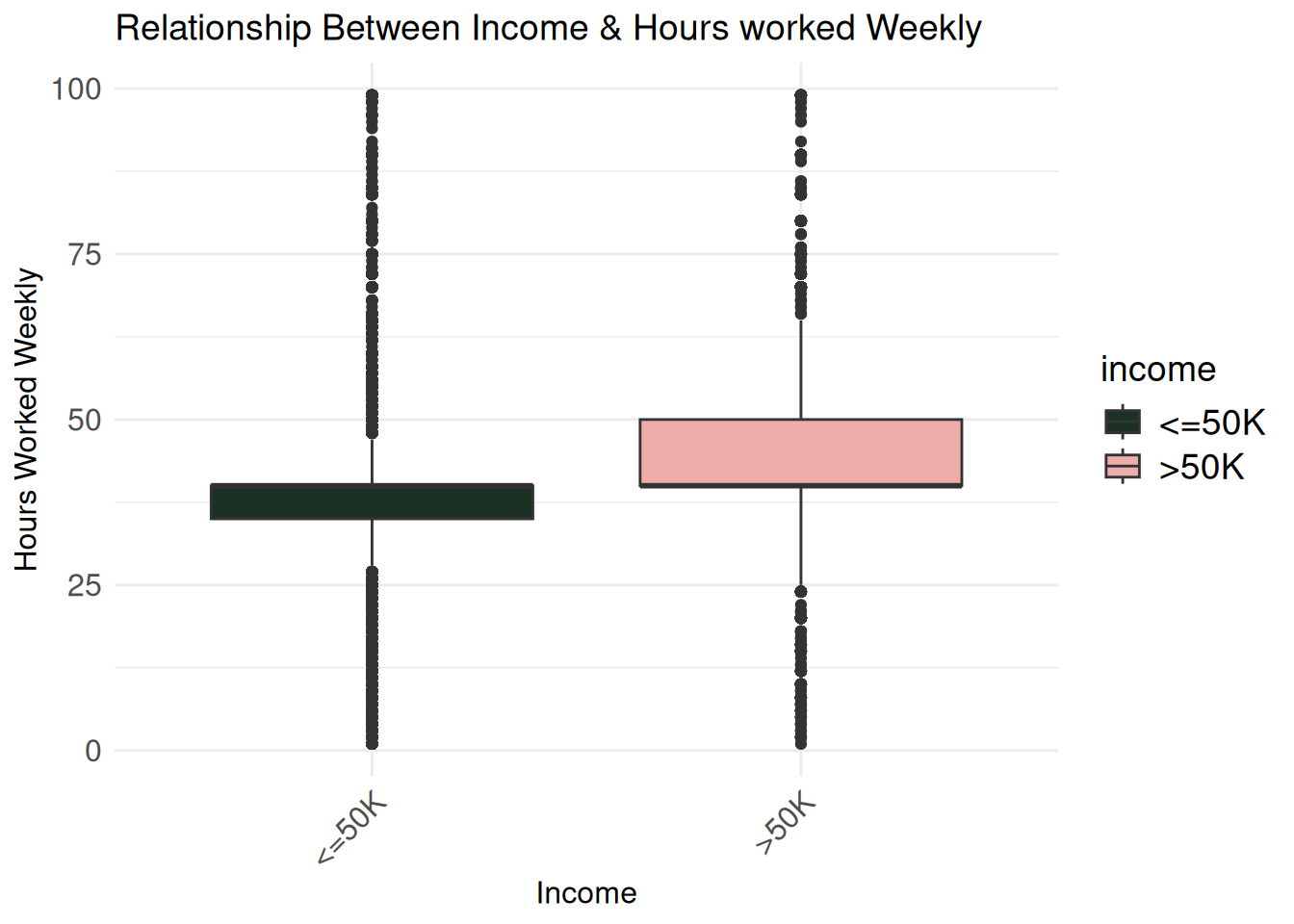
3.4 Bivariate Graphs

Six graphs might be a bit too much, but I found the following interesting: the income plotted against type of work, occupation, marital status, sex, age, and hours worked weekly. My eye-opening takeaways were that self-employed individuals with a registered incorporated business and people married to civillian spouses were more likely to make more than $50,000.

workclass_bivariate <- ggplot(census_eda, aes(x = workclass, 
                                              fill = income)) + 
  geom_bar(position = "fill") + 
  labs(
    title = "Relationship Between Income & Work Type",
    x = "Work Type",
    y = "Proportion of Observations") +
  theme_minimal() +
  scale_fill_wa_d("puget") +
  theme(
    axis.title.x = element_text(size = 12),
    axis.title.y = element_text(size = 12),
    axis.text.x = element_text(angle = 45, hjust = 1, size = 12),
    axis.text.y = element_text(size = 12),
    plot.title = element_text(size = 16),
    legend.title = element_text(size = 14),
    legend.text = element_text(size = 14))

occupation_bivariate <- ggplot(census_eda, aes(x = occupation, 
                                               fill = income)) + 
  geom_bar(position = "fill") + 
  labs(
    title = "Relationship Between Income & Occupation",
    x = "Occupation",
    y = "Proportion of Observations") +
  theme_minimal() +
  scale_fill_wa_d("puget") +
  theme(
    axis.title.x = element_text(size = 12),
    axis.title.y = element_text(size = 12),
    axis.text.x = element_text(angle = 45, hjust = 1, size = 12),
    axis.text.y = element_text(size = 12),
    plot.title = element_text(size = 16),
    legend.title = element_text(size = 14),
    legend.text = element_text(size = 14))

workclass_bivariate
occupation_bivariate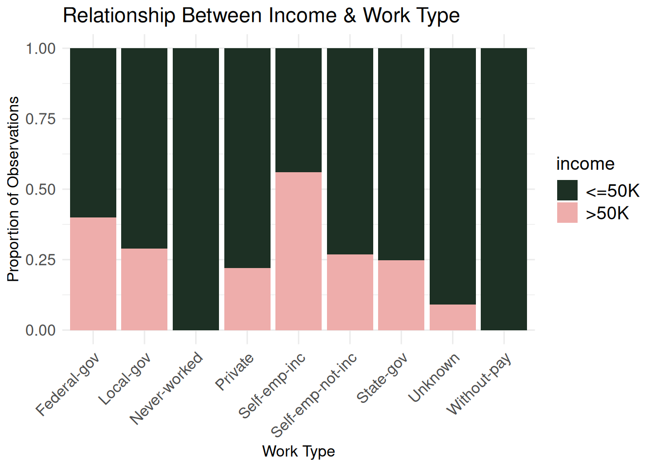

marriage_bivariate <- ggplot(census_eda, aes(x = marital.status, 
                                              fill = income)) + 
  geom_bar(position = "fill") + 
  labs(
    title = "Relationship Between Income & Marital Status",
    x = "Marital Status",
    y = "Proportion of Observations") +
  theme_minimal() +
  scale_fill_wa_d("puget") +
  theme(
    axis.title.x = element_text(size = 12),
    axis.title.y = element_text(size = 12),
    axis.text.x = element_text(angle = 45, hjust = 1, size = 12),
    axis.text.y = element_text(size = 12),
    plot.title = element_text(size = 16),
    legend.title = element_text(size = 14),
    legend.text = element_text(size = 14))

sex_bivariate <- ggplot(census_eda, aes(x = sex, 
                                               fill = income)) + 
  geom_bar(position = "fill") + 
  labs(
    title = "Relationship Between Income & Sex",
    x = "Sex",
    y = "Proportion of Observations") +
  theme_minimal() +
  scale_fill_wa_d("puget") +
  theme(
    axis.title.x = element_text(size = 12),
    axis.title.y = element_text(size = 12),
    axis.text.x = element_text(angle = 45, hjust = 1, size = 12),
    axis.text.y = element_text(size = 12),
    plot.title = element_text(size = 16),
    legend.title = element_text(size = 14),
    legend.text = element_text(size = 14))

marriage_bivariate
sex_bivariate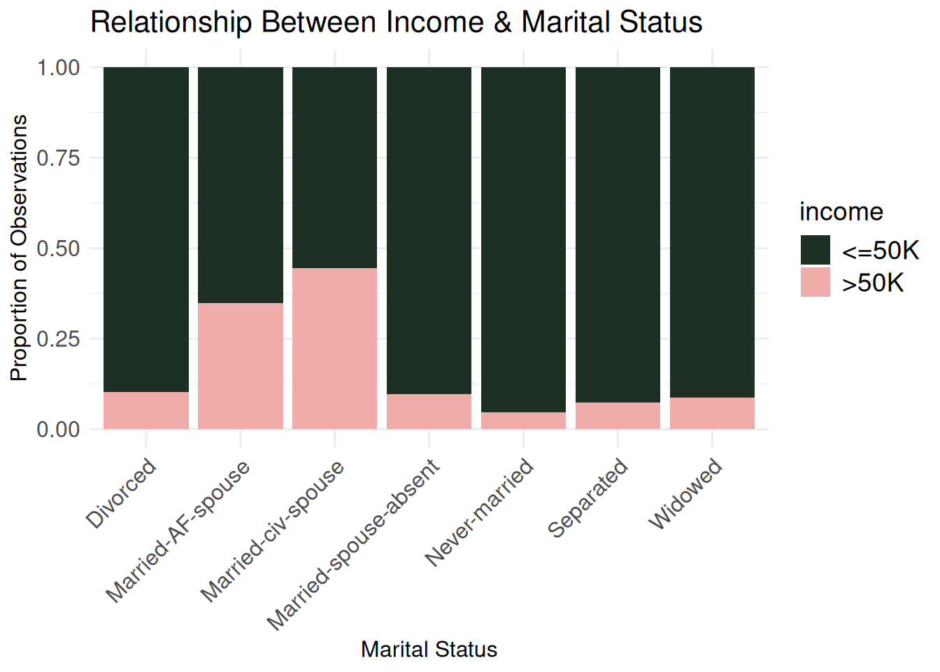

age_bivariate <- ggplot(census_eda, aes(x = income, y = age, fill = income)) +
  geom_boxplot() +
  labs(title = "Relationship Between Income & Age",
       x = "Income",
       y = "Age") +
  theme_minimal() +
  scale_fill_wa_d("puget") +
  theme(
    axis.title.x = element_text(size = 12),
    axis.title.y = element_text(size = 12),
    axis.text.x = element_text(angle = 45, hjust = 1, size = 12),
    axis.text.y = element_text(size = 12),
    plot.title = element_text(size = 14),
    legend.title = element_text(size = 14),
    legend.text = element_text(size = 14))

hours_bivariate <- ggplot(census_eda, aes(x = income, y = hours.per.week, fill = income)) +
  geom_boxplot() +
  labs(title = "Relationship Between Income & Hours worked Weekly",
       x = "Income",
       y = "Hours Worked Weekly") +
  theme_minimal() +
  scale_fill_wa_d("puget") +
  theme(
    axis.title.x = element_text(size = 12),
    axis.title.y = element_text(size = 12),
    axis.text.x = element_text(angle = 45, hjust = 1, size = 12),
    axis.text.y = element_text(size = 12),
    plot.title = element_text(size = 14),
    legend.title = element_text(size = 14),
    legend.text = element_text(size = 14))

age_bivariate
hours_bivariate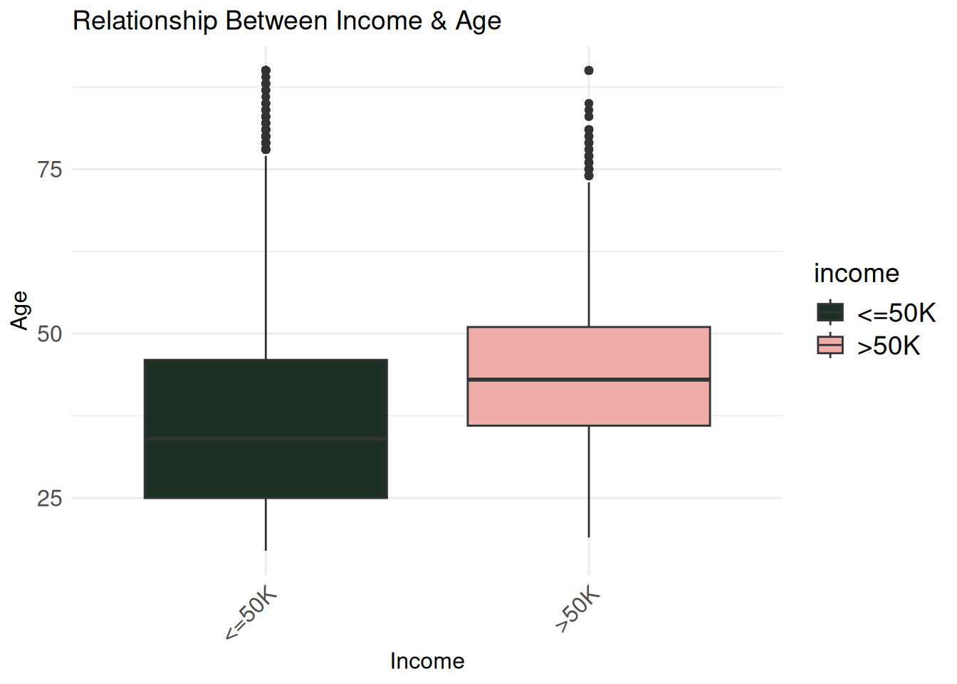

4 Model Management

4.1 Preparing Data for Modeling

I created an XGBoost model with the goal of tuning its hyperparameters for better performance.

boosted_model <- boost_tree(trees = tune(), 
                            learn_rate = tune(), 
                            tree_depth = tune(), 
                            min_n = tune()) |>
  set_engine("xgboost") |>
  set_mode("classification")

I treated ? values as NA so they could be imputed. I also converted categorical variables into factors, ensured numeric predictors were integers, used the median to impute numeric values, and the mode for categorical ones. Finally, I applied dummy (one-hot) encoding so categorical variables could be modeled numerically.

boosted_recipe <- recipe(income ~ ., data = census_train) |>
  step_mutate(across(where(is.character) | where(is.factor), ~ as.factor(stringr::str_trim(ifelse(as.character(.x) == "?", NA, as.character(.x)))))) |>
  step_indicate_na(all_predictors()) |>
  step_zv(all_predictors()) |>
  step_integer(all_numeric_predictors()) |>
  step_impute_median(all_numeric_predictors()) |>
  step_impute_mode(all_nominal_predictors()) |>
  step_dummy(all_nominal_predictors(), one_hot = TRUE)

I made a workflow to put our recipe and model together so they could easily be used with the training (and later the test) set.

boosted_workflow <- workflow() |>
  add_model(boosted_model) |>
  add_recipe(boosted_recipe)

I defined a grid of hyperparameter values for my XGBoost model using grid_space_filling(), which selects a diverse but efficient sample of combinations. I then applied 5-fold cross-validation (with one repeat) to evaluate each combination, stratifying by income to preserve class distribution across folds.

boosted_grid <- grid_space_filling(trees(range = c(20, 200)),
                                   tree_depth(range = c(1, 15)),
                                   learn_rate(range = c(-10,-1)),
                                   min_n(range = c(2, 40)),
                                   size = 50)

census_folds = vfold_cv(census_train, v = 5, repeats = 1, strata = income)

I used parallel processing to speed up tuning across my grid of hyperparameters. Using tune_grid(), I evaluated each model combination defined earlier using 5-fold cross-validation. The process was parallelized across 9 cores to reduce runtime, and the cluster was stopped afterward to free system resources.

cl <- makePSOCKcluster(9)
registerDoParallel(cl)

tuning_results <- tune_grid(
  boosted_workflow,
  resamples = census_folds,
  grid = boosted_grid
)

stopCluster(cl)

After tuning, I selected the hyperparameter combination that gave the highest accuracy and used it to train the final model.

boosted_fit <- boosted_workflow |>
  finalize_workflow(select_best(tuning_results, metric = "accuracy")) |>
  fit(census_train)

Finally, I used the tuned model to generate predictions on the test set. Since the test set didn’t include income labels, I converted the predicted class into a binary format (1 for “>50K”, 0 otherwise) and exported the results as a .csv file.

prediction_vector <- predict(boosted_fit, new_data = census_test, type = "class") |>
  mutate(income = ifelse(.pred_class %in% c(">50K", ">50K."), 1, 0)) |>
  select(income)

write.csv(prediction_vector, "my_predictions.csv", row.names = FALSE)

5 Final Thoughts

I don’t know :’).

5.1 Update

I came third (out of 15 people)!!! My accuracy was 86.6%. I will be returning to this in the near future because I am curious about pairing my stepwise BIC model WITH XGBoost and seeing what those results would be.

5.2 Limitations

I don’t really have anything to report on my final results. One reason is that while I had the test data, it actually does not have the income column. I will likely make an update here (once my teacher has evaluated my work) with my accuracy, and if possible, a confusion matrix and other metrics.

Gradient boosted trees are computationally expensive, meaning every mistake and consequent re-run cost me over 2 additional hours of runtime. That held me back from experimenting more, to be honest. I only repeated my cross-validation once as I suspect it would take 20+ hours if I did it 10 times (running my current setup with 1 fold took > 2 hours).

6 Reflection

I admittedly did not use my time wisely when doing this project, so I assume that under different circumstances I probably would have given certain decisions more thought (like increasing the number of repeats for cross validation, though I am unsure if that would necessarily benefit the accuracy) or had different solutions to certain problems. I do think, however, that I did a solid job, all things considered. I also learned the hard way about the importance of caching everything.